1. Meaning of the first parameter in SECTION 9 DESCRIPTION OF LINES

As explained in the manual the first parameter in SECTION 9: DESCRIPTION OF LINES in an integer which can have the values 0, 1, or 2. But it was only stated that options 1 and 2 are not fully implemented. That is why it is advisable to always use option 0 for all models, as we have done so far.

The reality is that now there are four usable options for the initial parameter: 0,1,2,3... This has been the case since many versions back (!). The meaning of this "mysterious" initial parameter of SECTION 9 is as follows:

0 = calculate the lines and their branches considering that the virtual extension of each line, intersects the midpoint of the N attachment points with which connects.
1 = calculate the lines and their branches considering that the virtual extension of each line, intersects the midpoint of the N attachment points with which connects, pondered by each chord length
2 = calculate the lines and their branches considering that the virtual extension of each line, intersects the midpoint of the N attachment points with which connects, pondered by each chord length and relative rib weight parameter set in column 7 of SECTION 2.
3 = calculate the lines and their branches considering that the virtual extension of each line, intersects the midpoint of the N attachement points with which connects, pondered by each chord length, the relative rib weight parameter set in column 7 of SECTION 2, and the distribution of loads in the attachement points of a rib according to the distribution selected in SECTION 18.

Option 0, is what we have used so far. It is the easiest to understand (simply each line naturally looks for the direction of the geometric center of the fixing points located on the sail). For example riser A is aligned with the geometric center of all attachments that connect to A. This is simply a conjecture, but it works, as shown in the real world.

Option 1, make a weighted average, considering only the chords lengths. That is, considering that the lift of each profile is proportional to the length of its chord. Of course, the central profiles support more load than those located towards the wing tips. Optimization spanwise.

Option 2, make a weighted average, considering the lengths of the chords and their relative weights, defined in column 7 of SECTION 2. Normally, the defined values are 1.0 (and can be defined as such, for all models). But, in some cases would be interesting to indicate relative weights of 2.0 or 3.0, when we use diagonals that allow to jump two or three cells and logically the load increases proportionally with respect to other zones with attachments in each profile (relative weight 1.0). Improved spanwise optimization.

Option 3, It is the most complete and recommended. Makes a weighted average using options 1 and 2, and also the percentage distribution of the loads in each profile, according to its number of attachments, according to SECTION 18. Thus, section 18 is not only used for elastic corrections and for informative calculation of loads at each attachment, but also for the perfect orientation of branches in space. In practice, using option 3 is very easy! Just type a "3" (instead of "0") in the first line of SECTION 9. The values given in section 18 can be considered invariant (approximate enough for all wings), although you can change to adjust to your preferences or profile types. The relative weights in column 7 of section 2 can be defined as "1.0" or slightly modified if you use mixed cell jumps. Optimization spanwise and chordwise.

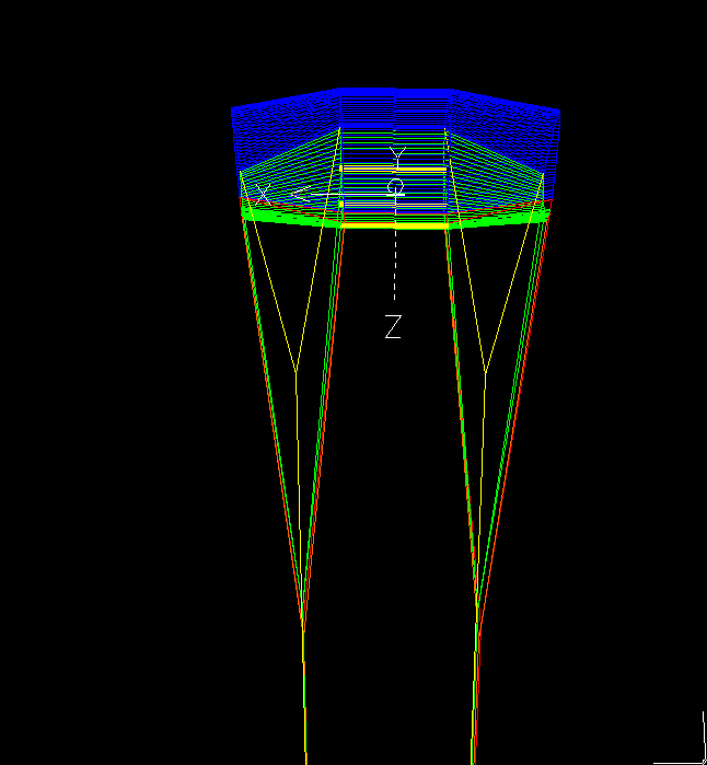
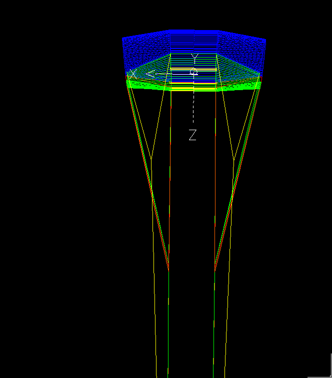
If you use option 3, it is also recommended to run the program once with option 0 to verify the differences. You can overlay 3D line models with different colors in the DXF 3D model or compare line listings. For example, in the case of the BHL5-16 model I checked for differences of up to 2.3 cm. It is expected that the calculation made with a weighted distribution type 3 will provide more solidity to the wing (without being able to quantify at this time the improvement obtained). In model gnuA6-32 the differences are up to 4 cm.

The ramifications of the brakes are always calculated by default according to model 0 (geometric), since the forces are applied directly by the pilot.

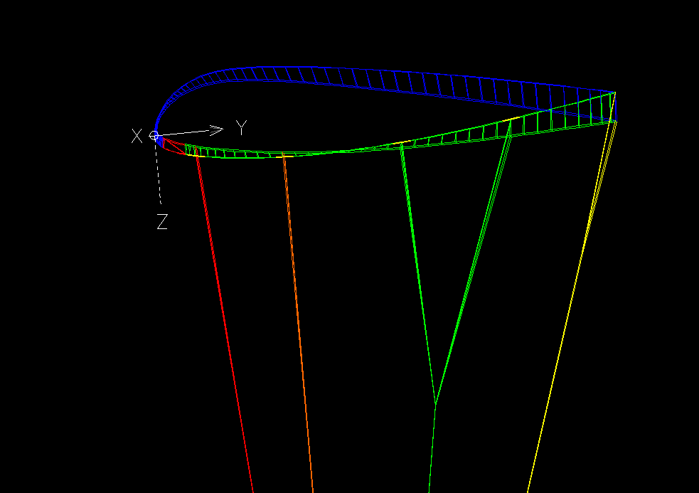
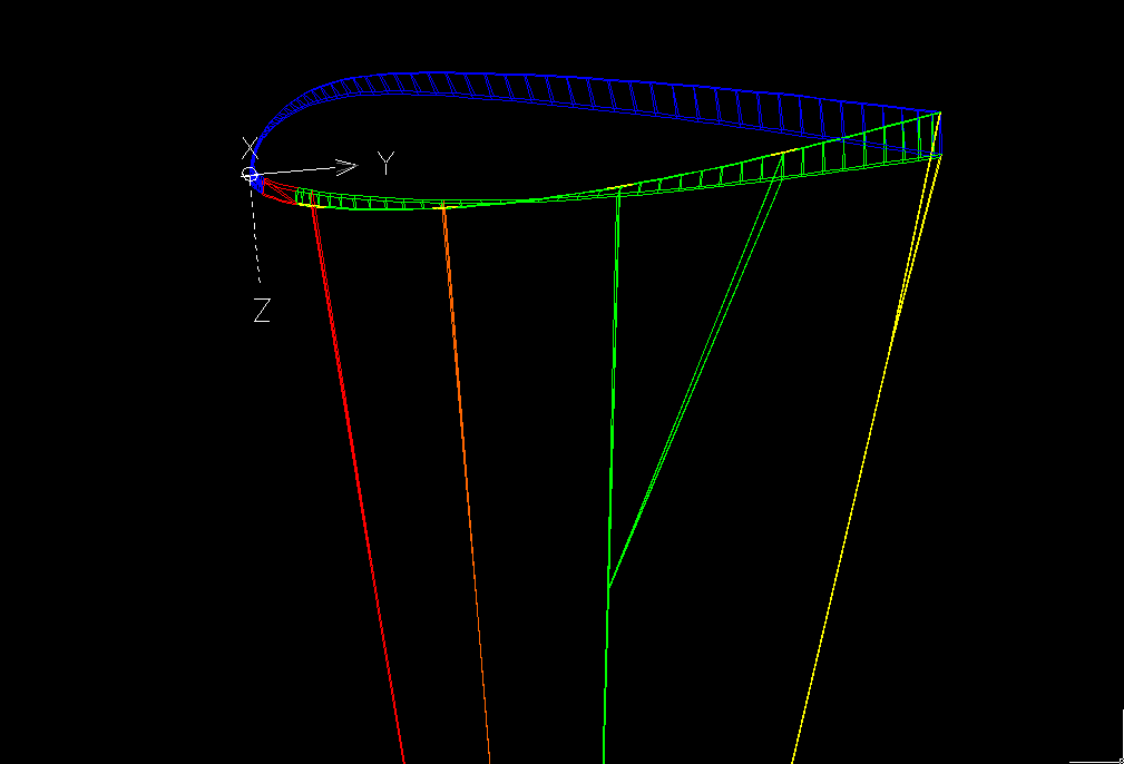
2. Minimal test example

We have created a minimal "paraglider" of only 3 cells and 4 ribs, to verify the effect of the parameters.

Input files:

gnuA.txt

leparagliding.txt

leparagliding Test 0 geometric.txt

leparagliding - Test 3 forced.txt

leparagliding - Test 3 natural.txt

***************************************************
*          9. SUSPENSION LINES DESCRIPTION
***************************************************
3                                                    <<< Parameter "3"
3
2
3    1 1    2 1    3 1    0 0     1 1
3    1 1    2 1    3 2    0 0     1 2
2
3    1 1    2 1    3 1    0 0     2 1
3    1 1    2 1    3 2    0 0     2 2
4
3    1 1    2 1    3 1    0 0     3 1
3    1 1    2 1    3 2    0 0     3 2
3    1 1    2 1    3 3    0 0     4 1
3    1 1    2 1    3 4    0 0     4 2

Forced sections:
**************************************************************
*             2. AIRFOILS                                *
**************************************************************
* Airfoil name, intake in, intake out, open , disp. rrw
1    gnua.txt    1.6    6.3    1    0    30    15        <<< relative rib weight 30 (!) in column 7. Normal vaule = 1.0
2    gnua.txt    1.6    6.3    0    0    1     1

Load distribution in % SECTION 18:
*****************************************************
*       18. Elastic lines corrections
*****************************************************
100
75    25                         <<< A=75% B=25% (2-liner)
40    40    20                   <<< A=40% B=40% C=20% (3-liner)
40    40    20    0              <<< A=40% B=40% C=20% D=0% (4-liner, forced; normal 35 35 20 10)
35    35    15    10    5        <<< A=35% B=35% C=15% D=10% E=5% (5-liner)
1    0.08    0.2    0.2   
2    0.08    0.2    0.2
3    0.08    0.2    0.2
4    0.08    0.2    0.2
5    0.08    0.2    0.2

Results:

Test 0 geometric lep-3d.dxf

Test 3 forced lep-3d.dxf

Test 3 natural lep-3d.dxf

01 Model parameter "0". Line C (green) passes through the geometric center of the attachments C and D.	02 Model parameter "3" forced using load distribution A=40% B=40% C=20% D=0%. Since it has been assumed that attachment D does not support load, the green bifurcation continues straight until C
03 Frontal Model 0.	04 Model type "3" forced using relative weight in rib 1 30 times higher than the rib 2 (exaggerated in order to verify the effect).
05 Comparative model "0" and model "3" natural in magenta (not forced). It makes sense for line C to move forward, since C attachment point supports less load than D.	06 Test 3 natural 3D

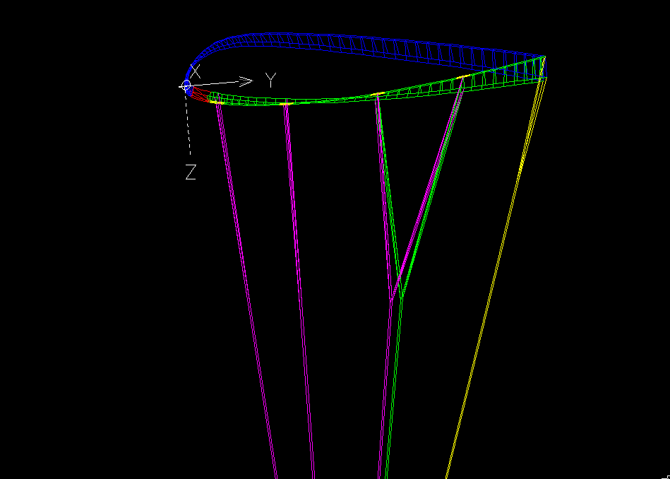
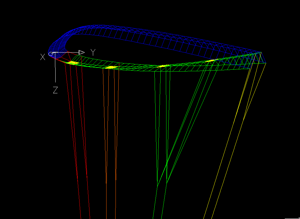
Parameters 0,1,2,3 now can be used with lep-3.16 and several previous versions. However it will be from lep-3.17 that it will be officially incorporated. Some additional checks need to be made, on the operation of the relative weights of column 7 of SECTION 2. Using values 1.0 in column 7 the results will already be very accurate. As stated above, it is recommended to compare with the simplified model 0 (figure 05).