le
PARAGLIDER DESIGN HANDBOOK
CHAPTER 5. PANEL FLAT DEVELOPMENT
 

5.1 Introduction
5.2 Description of the LE method
5.3 Analytical geometry principle
5.4 The FORTRAN subroutine

5.1 Introduction

This chapter describes the mathematical method for the flat development of the upper and lower panels of the cells.

Other designers use 3D modeling programs such as Rhino, 3dStudiomax ... but Laboratori d'envol algorithm has developed a small algorithm, very simple and giving the same, taken the airfoils in 3D directly from the CAD program.

5.2 Description of the LE method

1. The starting point is the 3D digital model of the paraglider with the airfoils in their relative position as planned.

2. We take two consecutive airfoils, which we call airfoil L (left) and airfoil R (right).

3. Each airfoil is divided into two curves (two 3D CAD polylines), corresponding to the upper surface (between LE and TE) and the corresponding to the lower surface (between LE and TE). Inlets are not part of these curves.

upper and lower surfaces
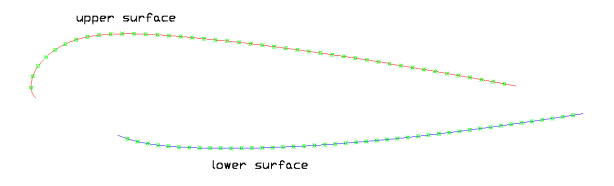
Fig 1: Upper and lower polylines of the airfoil

4. Take the upper left and upper right polylines, each of which is composed of N points, where N is large enough. Are the points from the initial definition of the airfoil. Running the CAD command "_list " on the polyline we obtained the coordinates x, y, z of the N points, that we copy to a text file, to be further processed by a subroutine.

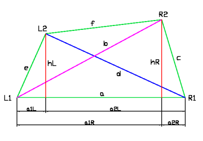
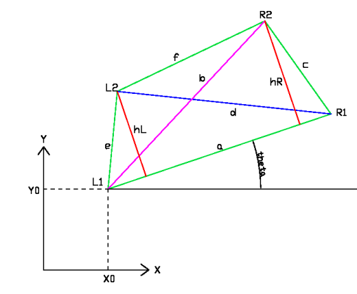
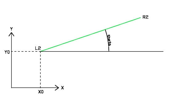
5. The basic idea is to take 2 consecutive points on the left L1, L2 and right R1, R2 to form a quadrilateral. Then we divide the quadrilateral (for one of its diagonal) into two triangles. We can calculate the sides of the triangles, because we know the coordinates of points. Then it is only required to develop the non planar quadrilater in a plane, placing the two triangles on a plane, articulated by the quadrilater diagonal. The error committed in the process is small, because the points are close and quadrilaterals are almost flat.

R-L airfoils
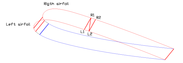
Fig. 2:  Two consecutive airfoils and reference points.

6. Repeat above process with the following points: L2 and L3, R2 and R3, and so on until the whole surface. The result is a flat surface developed from triangles with overlapping sides.

flat panel
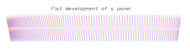
Fig. 3: Flat development

7. Repeat the process (4) with the L and R polylines of the lower surface.

8. Repeat the process (2) with all consecutive airfoils of the half wing.


5.3 Analytical geometry principle

This section describes the mathematical point (5) of the method outlined up.

quadrilater
Fig. 4: Study quadrilateral

Data:

L1, L2 Points of the left airfoil polyline
R1, R2 Points of the right airfoil polyline
a,b,c,d,e,f  distances between points

Unknowns:

hR= heigth of triangle L1-R1-R2
hL= heigth of triangle L1-R1-L2
a1R, a2R
a1L, a2L

Basic relations:

[1]    hR2+a1R2 = b2
[2]    hR2+a2R2 = c2
[3]    a1R + a2R = a

operand [1]-[2]:  

[4]    a1R2 - a2R2 = b2 - c2

replacing [3] in the previous ( a1R = a - a2R ) we obtain a2R :

[5]    a2R = ( a2 -b2 + c2 ) / ( 2*a )   and
[6]    a1R = a - a2R     and from [2]
[7]    hR = sqrt ( c2 - a2R2 )

and likewise for the other triangle:

[8]     a2L = ( a2 -e2 + d2 ) / ( 2*a )   and
[9]     a1L = a - a2L     and from [2]
[10]   hL = sqrt ( d2 - a2L2 )

Finally we have the flat coordinates of L1,L2,R1,R2 against an axes system orthogonal to L1-R1:

L1=(0,0)
R1=(a,0)
L2=(a1L,hL)
R2=(a1R,hR)

In the most general case, in an XY Cartesian coordinate system with the R1 at (x0, y0) and the segment L1-R1 inclined θ degrees inclined to the X-axis:

general
Fig. 5: General quadrilateral


L1x
L1y
=
X0
Y0

R1x
R1y
=
cos θ - sin θ
sin θ  cos θ
a
0
+
X0
Y0

L2x
L2y
=
cos θ - sin θ
sin θ  cos θ
a1L
hL
+
X0
Y0

R2x
R2y
=
cos θ - sin θ
sin θ  cos θ
a1R
hR
+
X0
Y0


Subsequent calculations are carried out with the rest of points 2-3, 3-4, 4-5, .... N-1-N taking in each step the following substitutions:

X0    <-------   L2x
Y0    <-------   L2y
tan θ = ( R2y -  L2y ) / ( R2x  - L2x )

steep
Fig. 5: Substitution and iteration


5.4 The FORTRAN subroutine

Reads the example files p1.txt and p2.txt (panel 7-8 upper from gnuLAB-1), and writes panell.dxf output.

c***************************************************************
c      PHC PARAGLIDING. PANEL SUBROUTINE.
c      Pere Hernàndez i Casellas
c      Laboratori d'envol
c      pere AT laboratoridenvol DOT com
c      Version 0.1 experimental 2005-02-13
c      Version 0.2 2006-09-01
c      Version 0.3 2009-01-10
c      FORTRAN g77 (GNU/Linux)
c***************************************************************

    program panell

    integer linecolor

    real rx(0:300),ry(0:300),rz(0:300)
    real sx(0:300),sy(0:300),sz(0:300)

    real x0,y0,theta

    real a,b,c,d,e,f

    real hr,a1r,a2r,hl,a1l,a2l

    real r1x(0:300),r1y(0:300),l1x(0:300),l1y(0:300)
    real r2x(0:300),r2y(0:300),l2x(0:300),l2y(0:300)

    area=0.

    open(unit=20,file='panel.dxf')
    open(unit=22,file='p1.txt')
    open(unit=23,file='p2.txt')

    rewind(22)
    rewind(23)

    pi=4.*atan(1.)

c   Read the left and right coordinates


    read (22,*)
    read (23,*)
    read (22,*) npunts
    read (23,*) npunts

    write (*,*) npunts

    do i=1,npunts

    read (22,*) x1,y1,z1
    read (23,*) x2,y2,z2

    rx(i)=x1
    ry(i)=y1
    rz(i)=z1
    sx(i)=x2
    sy(i)=y2
    sz(i)=z2

    write (*,*) rx(i),ry(i),rz(i)
    write (*,*) sx(i),sy(i),sz(i)

    end do

    x0=0.
    y0=0.
    theta=0.

    do i=1,npunts-1

c   Compute the basic lengths of the triangles

    a=sqrt((rx(i)-sx(i))*(rx(i)-sx(i))+(ry(i)-sy(i))*(ry(i)-sy(i))+(rz(i)-sz(i))*(rz(i)-sz(i)))
    b=sqrt((rx(i)-sx(i+1))*(rx(i)-sx(i+1))+(ry(i)-sy(i+1))*(ry(i)-sy(i+1))+(rz(i)-sz(i+1))*(rz(i)-sz(i+1)))
    c=sqrt((sx(i)-sx(i+1))*(sx(i)-sx(i+1))+(sy(i)-sy(i+1))*(sy(i)-sy(i+1))+(sz(i)-sz(i+1))*(sz(i)-sz(i+1)))
    d=sqrt((rx(i+1)-sx(i))*(rx(i+1)-sx(i))+(ry(i+1)-sy(i))*(ry(i+1)-sy(i))+(rz(i+1)-sz(i))*(rz(i+1)-sz(i)))
    e=sqrt((rx(i)-rx(i+1))*(rx(i)-rx(i+1))+(ry(i)-ry(i+1))*(ry(i)-ry(i+1))+(rz(i)-rz(i+1))*(rz(i)-rz(i+1)))
    f=sqrt((rx(i+1)-sx(i+1))*(rx(i+1)-sx(i+1))+(ry(i+1)-sy(i+1))*(ry(i+1)-sy(i+1))+(rz(i+1)-sz(i+1))*(rz(i+1)-sz(i+1)))

    write (*,*) a,f

    a2r=(a*a-b*b+c*c)/(2.*a)
    a1r=a-a2r
    hr=sqrt(c*c-a2r*a2r)

    a2l=(a*a-e*e+d*d)/(2.*a)
    a1l=a-a2l
    hl=sqrt(d*d-a2l*a2l)

    write(*,*) "a1,a2,a,a1+a2r", a1r,a2r,a,a1r+a2r
    write(*,*) "a1,a2,a,a1+a2l", a1l,a2l,a,a1l+a2l

    l1x(i)=x0
    l1y(i)=y0

    r1x(i)=a*cos(theta)+x0
    r1y(i)=a*sin(theta)+y0

    l2x(i)=a1l*cos(theta)-hl*sin(theta)+x0
    l2y(i)=a1l*sin(theta)+hl*cos(theta)+y0

    r2x(i)=a1r*cos(theta)-hr*sin(theta)+x0
    r2y(i)=a1r*sin(theta)+hr*cos(theta)+y0

    x0=l2x(i)
    y0=l2y(i)
    theta=atan((r2y(i)-l2y(i))/(r2x(i)-l2x(i)))

    write(*,*) "a1r,a2r,hr", a1r,a2r,hr
    write(*,*) "a1l,a2l,hl", a1l,a2l,hl

    write(*,*) x0,y0,theta

    end do

    do i=1,npunts-1

    write(*,*) l1x(i),l1y(i),l2x(i),l2y(i)

    call line(l1x(i),-l1y(i),r1x(i),-r1y(i),6)
    call line(l1x(i),-l1y(i),r2x(i),-r2y(i),5)
    call line(l1x(i),-l1y(i),l2x(i),-l2y(i),4)
    call line(r1x(i),-r1y(i),r2x(i),-r2y(i),3)
    call line(r1x(i),-r1y(i),l2x(i),-l2y(i),2)
    call line(l2x(i),-l2y(i),r2x(i),-r2y(i),3)

    end do
   
c   Close the output .dxf file

    write(20,'(A,/,I1,/,A)') "ENDSEC",0,"EOF"

c   Close units

    close (20)
    close (22)
    close (23)

    end

    SUBROUTINE line(p1x,p1y,p2x,p2y,linecolor)
c   line P1-P2
    integer linecolor
    write(20,'(A,/,I1,/,A)') "LINE",8,"default"
    write(20,'(I1,/,A)') 6,"CONTINUOUS"
    write(20,'(I2,/,F9.4,/,I2,/,F9.4)') 10,p1x,20,-p1y
    write(20,'(I2,/,F9.4,/,I2,/,F9.4)') 11,p2x,21,-p2y
    write(20,'(I2,/,I2,/,I2,/,I2,/,I2)') 39,0,62,linecolor,0

    return
    end