LE
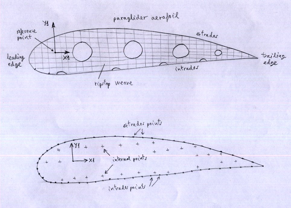
procedure to obtain the paraglider
aerofoil of any
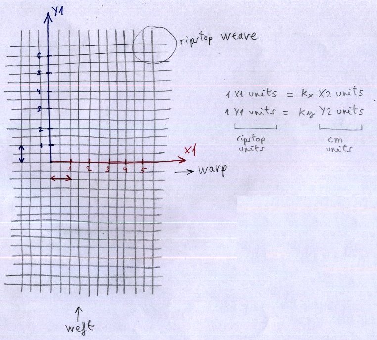
wing. Method based on the grid ripstop fabric
1. Auxiliary coordinate
system
2. Taking coordinates
3. Scale
corrections
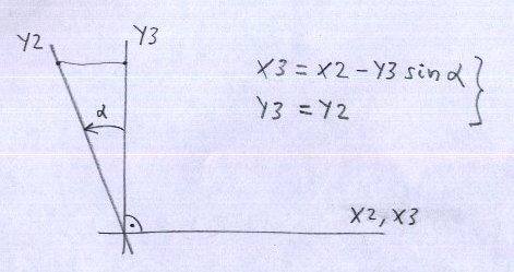
4. Orthogonality corrections
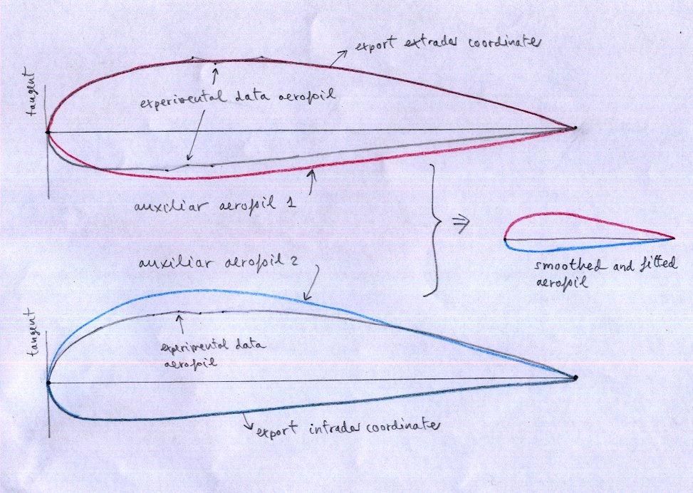
5. Normalization
6. Smoothing
7.
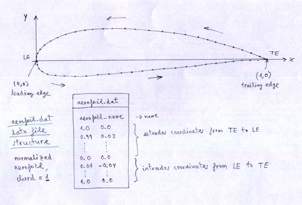
Note: ".dat" format